11 Clase 12

En esta clase vamos a centrarnos en el estudio e interpretación de variables categóricas en las regresión lineal.

Organización de la clase:

Presentaciones de a pares (10 mins. cada pareja)
Presentación de regresión logística

Esta es nuestra última clase y como instructora de la misma, estoy muy agradecida por su participación e interés en el curso. Todas sus opiniones sobre le curso en general y sobre mi desempeño en particular, serán bienvenidos en la aplicación de la universidad, a través de la encuesta de evaluación a profesores. Una vez más:

¡Gracias!

library(aod)
library(ggplot2)

mydata <- read.csv("https://stats.idre.ucla.edu/stat/data/binary.csv")

## view the first few rows of the data
head(mydata)

##   admit gre  gpa rank
## 1     0 380 3.61    3
## 2     1 660 3.67    3
## 3     1 800 4.00    1
## 4     1 640 3.19    4
## 5     0 520 2.93    4
## 6     1 760 3.00    2

summary(mydata)

##      admit             gre             gpa             rank      
##  Min.   :0.0000   Min.   :220.0   Min.   :2.260   Min.   :1.000  
##  1st Qu.:0.0000   1st Qu.:520.0   1st Qu.:3.130   1st Qu.:2.000  
##  Median :0.0000   Median :580.0   Median :3.395   Median :2.000  
##  Mean   :0.3175   Mean   :587.7   Mean   :3.390   Mean   :2.485  
##  3rd Qu.:1.0000   3rd Qu.:660.0   3rd Qu.:3.670   3rd Qu.:3.000  
##  Max.   :1.0000   Max.   :800.0   Max.   :4.000   Max.   :4.000

sapply(mydata, sd)

##       admit         gre         gpa        rank 
##   0.4660867 115.5165364   0.3805668   0.9444602

## two-way contingency table of categorical outcome and predictors we want
## to make sure there are not 0 cells
xtabs(~admit + rank, data = mydata)

##      rank
## admit  1  2  3  4
##     0 28 97 93 55
##     1 33 54 28 12

Using the logit model The code below estimates a logistic regression model using the glm (generalized linear model) function. First, we convert rank to a factor to indicate that rank should be treated as a categorical variable

mydata$rank <- factor(mydata$rank)
mylogit <- glm(admit ~ gre + gpa + rank, data = mydata, family = "binomial")

summary(mylogit)

## 
## Call:
## glm(formula = admit ~ gre + gpa + rank, family = "binomial", 
##     data = mydata)
## 
## Coefficients:
##              Estimate Std. Error z value Pr(>|z|)    
## (Intercept) -3.989979   1.139951  -3.500 0.000465 ***
## gre          0.002264   0.001094   2.070 0.038465 *  
## gpa          0.804038   0.331819   2.423 0.015388 *  
## rank2       -0.675443   0.316490  -2.134 0.032829 *  
## rank3       -1.340204   0.345306  -3.881 0.000104 ***
## rank4       -1.551464   0.417832  -3.713 0.000205 ***
## ---
## Signif. codes:  0 '***' 0.001 '**' 0.01 '*' 0.05 '.' 0.1 ' ' 1
## 
## (Dispersion parameter for binomial family taken to be 1)
## 
##     Null deviance: 499.98  on 399  degrees of freedom
## Residual deviance: 458.52  on 394  degrees of freedom
## AIC: 470.52
## 
## Number of Fisher Scoring iterations: 4

## CIs using profiled log-likelihood
confint(mylogit)

## Waiting for profiling to be done...

##                     2.5 %       97.5 %
## (Intercept) -6.2716202334 -1.792547080
## gre          0.0001375921  0.004435874
## gpa          0.1602959439  1.464142727
## rank2       -1.3008888002 -0.056745722
## rank3       -2.0276713127 -0.670372346
## rank4       -2.4000265384 -0.753542605

## CIs using standard errors
confint.default(mylogit)

##                     2.5 %       97.5 %
## (Intercept) -6.2242418514 -1.755716295
## gre          0.0001202298  0.004408622
## gpa          0.1536836760  1.454391423
## rank2       -1.2957512650 -0.055134591
## rank3       -2.0169920597 -0.663415773
## rank4       -2.3703986294 -0.732528724

wald.test(b = coef(mylogit), Sigma = vcov(mylogit), Terms = 4:6)

## Wald test:
## ----------
## 
## Chi-squared test:
## X2 = 20.9, df = 3, P(> X2) = 0.00011

l <- cbind(0, 0, 0, 1, -1, 0)
wald.test(b = coef(mylogit), Sigma = vcov(mylogit), L = l)

## Wald test:
## ----------
## 
## Chi-squared test:
## X2 = 5.5, df = 1, P(> X2) = 0.019

## odds ratios only
exp(coef(mylogit))

## (Intercept)         gre         gpa       rank2       rank3       rank4 
##   0.0185001   1.0022670   2.2345448   0.5089310   0.2617923   0.2119375

## odds ratios and 95% CI
exp(cbind(OR = coef(mylogit), confint(mylogit)))

## Waiting for profiling to be done...

##                    OR       2.5 %    97.5 %
## (Intercept) 0.0185001 0.001889165 0.1665354
## gre         1.0022670 1.000137602 1.0044457
## gpa         2.2345448 1.173858216 4.3238349
## rank2       0.5089310 0.272289674 0.9448343
## rank3       0.2617923 0.131641717 0.5115181
## rank4       0.2119375 0.090715546 0.4706961

newdata1 <- with(mydata, data.frame(gre = mean(gre), gpa = mean(gpa), rank = factor(1:4)))

## view data frame
newdata1

##     gre    gpa rank
## 1 587.7 3.3899    1
## 2 587.7 3.3899    2
## 3 587.7 3.3899    3
## 4 587.7 3.3899    4

newdata1$rankP <- predict(mylogit, newdata = newdata1, type = "response")
newdata1

##     gre    gpa rank     rankP
## 1 587.7 3.3899    1 0.5166016
## 2 587.7 3.3899    2 0.3522846
## 3 587.7 3.3899    3 0.2186120
## 4 587.7 3.3899    4 0.1846684

newdata2 <- with(mydata, data.frame(gre = rep(seq(from = 200, to = 800, length.out = 100),
    4), gpa = mean(gpa), rank = factor(rep(1:4, each = 100))))
    
    
newdata3 <- cbind(newdata2, predict(mylogit, newdata = newdata2, type = "link",
    se = TRUE))
newdata3 <- within(newdata3, {
    PredictedProb <- plogis(fit)
    LL <- plogis(fit - (1.96 * se.fit))
    UL <- plogis(fit + (1.96 * se.fit))
})

## view first few rows of final dataset
head(newdata3)

##        gre    gpa rank        fit    se.fit residual.scale        UL        LL
## 1 200.0000 3.3899    1 -0.8114870 0.5147714              1 0.5492064 0.1393812
## 2 206.0606 3.3899    1 -0.7977632 0.5090986              1 0.5498513 0.1423880
## 3 212.1212 3.3899    1 -0.7840394 0.5034491              1 0.5505074 0.1454429
## 4 218.1818 3.3899    1 -0.7703156 0.4978239              1 0.5511750 0.1485460
## 5 224.2424 3.3899    1 -0.7565919 0.4922237              1 0.5518545 0.1516973
## 6 230.3030 3.3899    1 -0.7428681 0.4866494              1 0.5525464 0.1548966
##   PredictedProb
## 1     0.3075737
## 2     0.3105042
## 3     0.3134499
## 4     0.3164108
## 5     0.3193867
## 6     0.3223773

ggplot(newdata3, aes(x = gre, y = PredictedProb)) + geom_ribbon(aes(ymin = LL,
    ymax = UL, fill = rank), alpha = 0.2) + geom_line(aes(colour = rank),
    size = 1)

## Warning: Using `size` aesthetic for lines was deprecated in ggplot2 3.4.0.
## ℹ Please use `linewidth` instead.
## This warning is displayed once every 8 hours.
## Call `lifecycle::last_lifecycle_warnings()` to see where this warning was
## generated.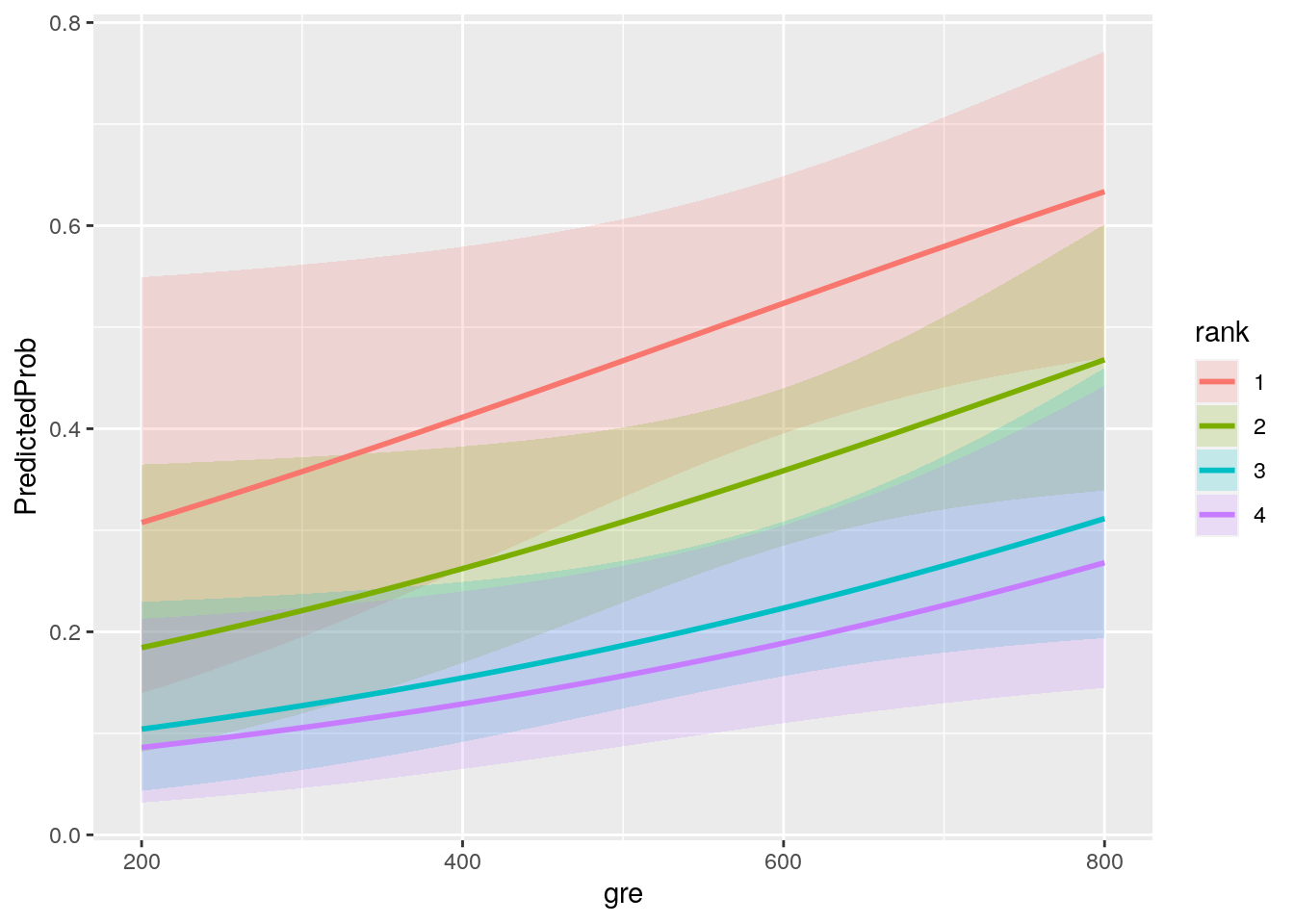

with(mylogit, null.deviance - deviance)

## [1] 41.45903

with(mylogit, df.null - df.residual)

## [1] 5

with(mylogit, pchisq(null.deviance - deviance, df.null - df.residual, lower.tail = FALSE))

## [1] 7.578194e-08

logLik(mylogit)

## 'log Lik.' -229.2587 (df=6)

Tips para el análisis:

Regresión lineal:

“Si X1 varía en 1 unidad [ver unidades de la variable], la Variable Dependiente cambia (se incrementa o decrece, según el signo del coeficiente) en B1 unidades, ceteris paribus.”

El R2 indica cuánto de Y está explicado por la/s variables del modelo. Se interpreta en %, debo multiplicar el resultado de R2*100. Ejemplo: R2: 0.2. “El 20% de las notas de los estudiantes está explicado por la influencia de las horas de estudio.” Es decir, que el efecto marginal de la

Regresión logística:

De los coeficientes sólo podemos interpretar el signo (+ o -) que indican la dirección de la relación. Pero no su magnitud. Para obtener la magnitud de la relación se necesita obtener los efectos marginales.